The Variational Autoencoder as a Two-Player Game — Part II

Variational Return to the Autoencoding Olympics

Welcome to Part II of this three part series on variational autoencoders and their application to encoding text.

In Part I we followed our two contestants Alice and Bob as they were training for the Autoencoding Olympics. We learned about the basics of autoencoders, as well as deep learning in general, and what kind of codes Alice and Bob might learn.

We also saw that the traditional autoencoder comes with the risk of memorisation instead of true learning. This ultimately lead to Alice and Bob messing up their performance at the Olympics when they encountered data they had never seen before.

Introducing the Variational Autoencoder (VAE)

Returning home completely depressed from their disastrous performance at the Autoencoding Olympics, Alice and Bob regroup and think how they can change their approach for the next Games.

Because their experience was so catastrophic and embarrassing, not getting a single test image they were given even remotely correct, they decide to start completely from scratch.

So Alice and Bob throw out the code they came up with and go on an epic drinking spree, erasing absolutely everything they had learned so far from their mind.

Tabula rasa.

Their minds are completely blank again. Just like when we first met them.

After recovering from their equally epic hangovers, they decide to upgrade their autoencoding devices to a newer model they recently heard about. A variational model.

The variational model is only recommended for expert encoder/decoder pairs. And it’s only intended for training. It actually makes the process more difficult. But Alice and Bob want to be at the top of their game after all.

No pain no gain.

The original devices were really just a pair of senders and receivers for code and feedback respectively. The new devices are slightly different. Let’s look at how they work.

Alice still inputs the code that she thinks is most likely. But in addition, she also has to enter an uncertainty!

Based on this, the machine doesn’t directly transfer the value Alice puts in as most likely to Bob. Instead, it chooses a random number according to the distribution she entered.

It randomly samples Alice’s code distribution.

So Bob still only gets a single number per code dimension. But this number has now acquired a bit of randomness in the process of being transferred from Alice’s machine to Bob’s.

Actually, one of the main contributions of the original paper introducing the VAE was a trick (called the “reparametrization trick”) that allowed Bob to give useful feedback to Alice despite not knowing the exact values Alice chose, but only the randomized ones the machine passed on to him.

In principle Alice can still choose to enter very low uncertainties so that Bob almost certainly gets the exact value she wants to transmit.

But the catch is that Charlie has become stricter.

He now also subtracts a penalty from their score. The smaller an uncertainty Alice chooses, the larger the penalty Charlie applies.

If Alice is confident that even a value that’s only kind of close to her desired one still conveys all the information, she can choose a higher uncertainty and sacrifice less of their score.

On the other hand, if the code needs to be very precise to convey the image to Bob, Alice needs to choose a low uncertainty. This way, even if Bob perfectly reconstructs the image and earns them a perfect score, they loose a lot of it due to the uncertainty penalty.

This forces Alice and Bob to be smarter about the code they choose. It needs to be more robust against small changes. Even if the code gets distorted a bit in transmission, Bob should still paint a fairly similar painting.

Smoothing out the Code

Let’s look at the extreme example of encoding with only a single number again.

We saw in Part I that without uncertainty, Alice and Bob could just learn to associate a unique code number with each of their training images, basically memorising their entire training dataset.

In one particular code, Alice could just encode consecutively numbered images with a code separated by 0.000001. Image 156 would correspond to code 0.000156, image 157 to 0.000157, and so on. Irrespective of what these images actually contain.

If Bob gets the exact number, he has learned through many iterations of trial and error exactly the corresponding image he has to paint.

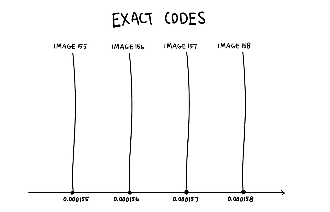
The problem is that this creates “holes” in the code. Alice never encodes anything in the spaces between for example 0.000156 and 0.000157. Thus any number in these gaps, say 0.0001561 or 0.0001568, is absolutely meaningless to Bob.

Sure, he could round up or down to the nearest number he associates with an image, but that will mean there is a sharp transition in their code at places like 0.0001565. The tiniest change in the code number could mean Bob has to paint a completely different image.

Their code is not smooth.

It also cannot be used to encode unfamiliar images without further training and modification. This is what lead to their downfall in Part I. Their code didn’t generalise. They were overfitting to the training data.

However, as Alice starts using small amounts of uncertainty, she starts “filling in the holes”, smoothing out their code a little bit.

If she wants to send image 156 and enters 0.000156 with a small uncertainty, Bob will get a number that’s close to it, but most likely not exactly the same.

And as they play the same game many times with the same image, even if Alice’s code doesn’t change, Bob will still see several slightly different numbers associated with each image.

This already helps them being less reliant on precise numbers.

But such small uncertainty still comes with a high penalty!

If they really want to succeed and get a good overall score from Charlie, they need to figure out how to come up with a code that is robust to much higher uncertainty.

If Alice still wants to encode Image 156 at 0.000156 and Image 157 at 0.000157 she better make sure that those two images are almost identical unless they want to sacrifice a huge amount of their score by choosing a tiny uncertainty.

So unless those two images are actually really similar, this code is incredibly wasteful and should be avoided.

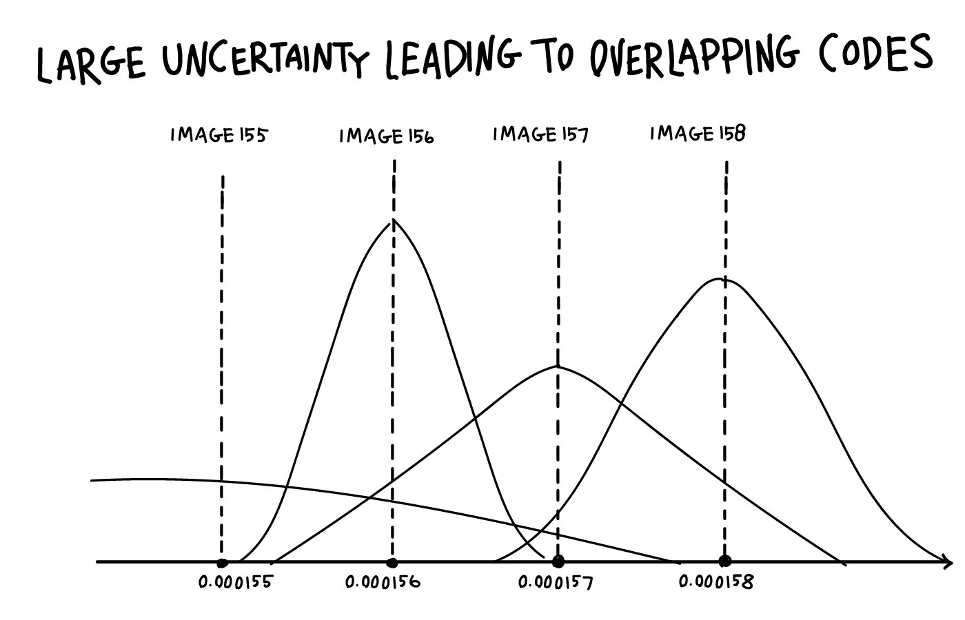
If the uncertainty is not significantly smaller than 0.000001, there is a considerable chance that even though Alice wants to encode image 157, the machine actually sends the code she would have chosen for image 156 to Bob. Or something even more different.

Then, even if Bob understands Alice’s ideal code, he will still paint the wrong image. If they want to get a high score while maintaining a low penalty they have to learn to encode similar images with a similar code.

Towards Meaningful Codes

Back to the full game with a two dimensional code, we can also think of this in a slightly different way. Instead of encoding each image into a single point in our 2-D plane, Alice now has to encode them into little smudges. The smaller the smudge, the higher the penalty.

You can cram infinitely many points into even a tiny space.

Smudges on the other hand will soon start to overlap, so you better make sure that the overlaps kind of make sense.

Using this new machine and Charlie’s stricter scoring prevents them from just memorizing the training data. They need to give actual meaning to their code.

This forces them to come up with a code that’s smooth, or continuous, so neighboring regions in “code space” (also called “latent space”) encode very similar images in “data space”. This way they don’t sacrifice too much of their score by having to specify the point very accurately with low uncertainty.

This naturally leads to clustering in code space.

The improved code they learned carries much more meaning. Instead of encoding images directly, which is both wasteful and fragile, the code actually contains more abstract ideas, just like we discussed in Part I.

In one region we might find images of white Chihuahuas in the bottom right of the photo, in another region are all the images of black cats playing with a ball at the centre of the photo, and so on. All transitioning as smoothly as possible, so that neighboring images are as similar as possible.

Leaving the world of Alice and Bob for a moment, Laurens van der Maaten and Geoffrey Hinton produced a nice visualization of this kind of clustering (although using a very different technique called t-SNE) for the famous MNIST dataset, comprising many different images of the digits 0 to 9.

We see that similar digits cluster together, for example zeros in the bottom left. But even more, within each digit cluster, we see similar styles (e.g. slant, stroke width,…) clustering together.

Back to Alice and Bob.

Armed with their new experience gained from the variational training, they return to the next Autoencoding Olympics. Here they simply revert to their old strategy where Alice directly passes on the code without any uncertainty.

But crucially, they use the new code learned through variational training.

And the training paid off!

With this code, they ace images they have never encountered in training and completely destroy their competition.

Playtime

To celebrate their victory, they play around with their learned code a bit. They discover some very interesting tricks they can now perform.

The first one allows them to smoothly interpolate between real photos.

They can encode two real images, getting a code for each, and then smoothly go from one to the other by taking intermediate codes and having Bob decode them.

As a simple example, let’s assume they repeat their training with images of people, and then encode photos of themselves, one of Alice and one of Bob. For the sake of example, let’s just say those codes happen to be (0.0, 3.0) for Alice and (6.0, 0.0) for Bob.

They can now continuously transition between them.

Let’s say they decode two equally spaced intermediate images. Those intermediate images would be at (2.0, 2.0) and (4.0, 1.0).

As Bob decodes them they see that the the photo at (2.0, 2.0) is basically 66.6% Alice and 33.3% Bob, and the one at (4.0, 1.0) has the opposite ratio, 33.3% Alice and 66.6% Bob.

But crucially it’s not just the original photos superimposed like you could easily do in Photoshop. It’s really what a photo of a person that’s “One third Alice and two thirds Bob” might look like.

In this way, VAEs allow for the creation of absolutely realistic looking data that does not exist in the real world. We could for example encode photos of ourselves and our partner and interpolate between them to guess what our kids might look like (assuming they also turn out to be some kind of gender-hybrid).

For a real example of photo interpolations, check out this extremely trippy video of interpolations between faces of celebrities.

And this is not limited to images. As we will see in the next part, we can encode other types of data too. We could imagine encoding two songs we like and listen to what various interpolations between those two might sound like. Or as the Magenta team has shown with their NSynth project, we could interpolate between different musical instruments.

All this also opens up tremendous artistic opportunities. For some great examples, take a look at hardmaru’s interpolations between human-made sketches as well as much of his other work. His Instagram account is a wonderful source of AI generated art using techniques very similar to the one Alice and Bob are using.

Another interesting trick they discover is that by modifying their training process a bit, they can actually give a particular meaning to one or more of their code dimensions. This is similar to the simple dog/cat and black/white code we discussed in Part I where both dimensions had a clearly human-interpretable meaning.

For example they could use one dimension to encode the very particular property of beard length.

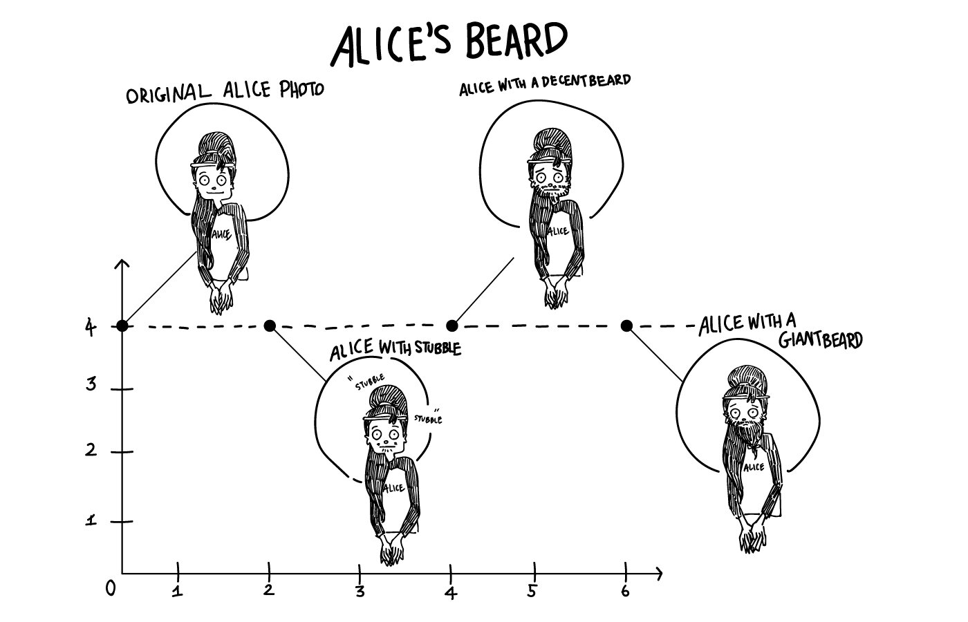
Let’s assume they use the first dimension for beard length, with 0 meaning no beard, and the larger the number the longer the beard.

Alice again encodes an image of herself. Naturally, Alice not being a bearded lady, this has value 0.0 for the first code number.

Let’s assume that it happens to be encoded at (0.0, 4.0) in this new code. Bob can now do something interesting. He can paint images he would associate with codes at (X, 4.0). The larger X, the longer the beard, while keeping the other code dimension fixed will preserve the “Aliceness” of the image. So he can basically realistically predict what Alice would look like with beards of various lengths.

For a real world example of this, have a look at the data generated by the InfoGAN proposed by Xi Chen and collaborators. This paper uses a different generative model, a so called Generative Adversarial Network (GAN), but the basic idea is the same. The state of the art has improved tremendously and the images that can be generated have become much more detailed and realistic, but this was one of the early papers pioneering this idea.

That was fun! But enough playing around. Alice and Bob need to focus again. They already have a new goal in mind!

In the final part of this series we will follow their journey back to the Autoencoding Olympics. This time in a new discipline: Text Encoding.